Running Legate Programs

Python programs using the Legate APIs (directly or through a Legate-based library such as cuPyNumeric) can be run using the standard Python interpreter:

$ python myprog.py <myprog.py options>

By default this invocation will use most of the hardware resources (e.g. CPU cores, RAM and GPUs) available on the current machine, but this can be controlled, see Resource Allocation.

You can also use the custom legate driver script, that makes configuration easier, and offers more execution options, particularly for Distributed Launch:

$ legate myprog.py <myprog.py options>

Compiled C++ programs using the Legate API can also be run using the legate driver:

$ legate ./myprog <myprog options>

or invoked directly:

$ ./myprog <myprog options>

Runtime Configuration

Legate does not consume any command-line options. Instead, it is configured by a single environment variable, LEGATE_CONFIG which accepts a space-separated string of arguments:

$ LEGATE_CONFIG='--cpus=2 --gpus=10 --fbmem=1024' ./myprog

Important

LEGATE_CONFIG is read exactly once, during the first call to legate::start() (or first time importing the legate.core module in Python). Modifying LEGATE_CONFIG at any point after this call will have no effect. Calling legate::start() multiple times will also have no effect.

The user may query the flags available for configuration by passing the --help flag:

$ LEGATE_CONFIG='--help' ./myprog

This will cause Legate to list the available runtime options and exit the program.

Boolean flags may take several forms:

• --flag: implies flag=true.

• --flag=1|t|true|y|yes: implies flag=true.

• --flag=0|f|false|n|no: implies flag=false.

While the = separator between the flag’s name and value is optional (--flag=value is equivalent to --flag value), it is nevertheless recommended in order to make value association clearer.

The same flag (regardless of type) may also be passed multiple times to LEGATE_CONFIG, with the last value “winning”. For example:

$ LEGATE_CONFIG='--foo --foo=f --foo=1'

is equivalent to:

$ LEGATE_CONFIG='--foo=1'

Resource Allocation

By default Legate will query the available hardware on the current machine, and reserve for its use all CPU cores, all GPUs and most of the available memory. You can use --show-config (as a flag to the legate driver script, or through LEGATE_CONFIG) to inspect the exact set of resources that Legate decided to reserve. You can fine-tune Legate’s default resource reservation by passing specific flags to legate / LEGATE_CONFIG, listed later in this section.

You can also use --auto-config=0 to disable Legate’s automatic configuration. In this mode Legate will only reserve a minimal set of resources (only 1 CPU core for task execution, no GPUs, minimal system memory allocation), and any increases must be specified manually.

The following legate / LEGATE_CONFIG flags control how many processors are used by Legate:

• --cpus: how many individual CPU threads are spawned

• --omps: how many OpenMP groups are spawned

• --ompthreads: how many threads are spawned per OpenMP group

• --gpus: how many GPUs are used

The following flags control how much memory is reserved by Legate:

• --sysmem: how much DRAM (in MiB) to reserve

• --numamem: how much NUMA-specific DRAM (in MiB) to reserve per NUMA node

• --fbmem: how much GPU memory (in MiB) to reserve per GPU

Pass --help to legate / LEGATE_CONFIG for a full list of accepted configuration options.

For example, if you wanted to use only part of the resources on a DGX station, you might run your application as follows:

$ legate --gpus 4 --sysmem 1000 --fbmem 15000 myprog.py

This will make only 4 of the 8 GPUs available for use by Legate. It will also allow Legate to consume up to 1000 MiB of DRAM and 15000 MiB of each GPU’s memory for a total of 60000 MiB of GPU memory.

The same configuration can also be passed through the environment variable LEGATE_CONFIG:

$ LEGATE_CONFIG="--gpus 4 --sysmem 1000 --fbmem 15000" legate myprog.py

including when using the standard Python interpreter:

$ LEGATE_CONFIG="--gpus 4 --sysmem 1000 --fbmem 15000" python myprog.py

or when running a compiled C++ Legate program directly:

$ LEGATE_CONFIG="--gpus 4 --sysmem 1000 --fbmem 15000" ./myprog

To see the full list of arguments accepted in LEGATE_CONFIG, you can pass LEGATE_CONFIG="--help":

$ LEGATE_CONFIG="--help" ./myprog

You can also allocate resources when running in interactive mode (by not passing any *.py files on the command line):

$ legate --gpus 4 --sysmem 1000 --fbmem 15000
Python 3.12.4 | packaged by conda-forge | (main, Jun 17 2024, 10:23:07) [GCC 12.3.0] on linux
Type "help", "copyright", "credits" or "license" for more information.
>>>

Note

Currently Legate assumes that all GPUs have the same memory capacity. If this is not the case, you should manually set --fbmem to a value that is appropriate for all devices, or skip the lower-memory devices using CUDA_VISIBLE_DEVICES. E.g. if GPU 1 has low memory capacity, and you only wish to use GPUs 0 and 2, you would use CUDA_VISIBLE_DEVICES=0,2.

Distributed Launch

You can run your program across multiple nodes by using the --nodes option followed by the number of nodes to be used. When doing a multi-process run, a launcher program must be specified, that will do the actual spawning of the processes. Run a command like the following from the same machine where you would normally invoke mpirun:

$ legate --nodes 2 --launcher mpirun --cpus 4 --gpus 1 myprog.py

In the above invocation the mpirun launcher will be used to spawn one Legate process on each of two nodes. Each process will use 4 CPU cores and 1 GPU on its assigned node.

The default Legate conda packages include networking support based on UCX, but GASNet-based packages are also available.

Note that resource setting flags such as --cpus 4 and --gpus 1 refer to each process. In the above invocation, each one of the two launched processes will reserve 4 CPU cores and 1 GPU, for a total of 8 CPU cores and 2 GPUs across the whole run.

Check the output of legate --help for the full list of supported launchers.

You can also perform the same launch as above externally to legate:

$ mpirun -n 2 -npernode 1 legate --cpus 4 --gpus 1 myprog.py

or use python directly:

$ LEGATE_CONFIG="--cpus 4 --gpus 1" mpirun -n 2 -npernode 1 -x LEGATE_CONFIG python myprog.py

Multiple processes (“ranks”) can also be launched on each node, using the --ranks-per-node legate option:

$ legate --ranks-per-node 2 --launcher mpirun myprog.py

The above will launch two processes on the same node (the default value for --nodes is 1).

Because Legate’s automatic configuration will not check for other processes sharing the same node, each of these two processes will attempt to use the full set of CPU cores on the node, causing contention. Even worse, each process will try to reserve most of the system memory in the machine, leading to a memory reservation failure at startup.

To work around this, you will want to explicitly reduce the resources requested by each process:

$ legate --ranks-per-node 2 --launcher mpirun --cpus 4 --sysmem 1000 myprog.py

With this change, each process will only reserve 4 CPU cores and 1000 MiB of system memory, so there will be enough resources for both.

Even with the above change contention remains an issue, as the processes may end up overlapping on their use of CPU cores. To work around this, you can explicitly partition CPU cores between the processes running on the same node, using the --cpu-bind legate option:

$ legate --ranks-per-node 2 --launcher mpirun --cpus 4 --sysmem 1000 --cpu-bind 0-15/16-32 myprog.py

The above command will restrict the first process to CPU cores 0-15, and the second to CPU cores 16-32, thus removing any contention. Each process will reserve 4 out of its allocated cores for task execution.

You can similarly restrict processes to specific NUMA domains, GPUs and NICs using --mem-bind, --gpu-bind and --nic-bind respectively.

You can also launch multiple processes per node when doing an external launch, but you then have to manually control the binding of resources:

$ mpirun -n 2 -npernode 2 --bind-to socket legate --cpus 4 --sysmem 1000 myprog.py

The above will launch two processes on one node, and relies on mpirun to bind each process to a separate CPU socket, thus partitioning the CPU cores between them.

Running Legate on Typical SLURM Clusters

Here is an example showing how to run Legate programs on typical SLURM clusters.

To get started, create a conda environment and install Legate, following the installation guide:

$ conda create -n legate -c conda-forge -c legate legate

For interactive runs, here are the steps:

Use srun from the login node to allocate compute nodes:

$ srun --exclusive -J <job-name> -p <partition> -A <account> -t <time> -N <nodes> --pty bash

Once the compute nodes are allocated, use the legate driver script to launch applications:

$ source "<path-to-conda>/etc/profile.d/conda.sh"  # Needed if conda isn't already loaded
$ conda activate legate
$ legate --launcher mpirun --verbose prog.py

You need to ensure the correct launcher is specified for your cluster. Some SLURM clusters support both srun and mpirun, while others only support srun.

The driver script should be able to infer the number of nodes to launch over, by reading environment variables set by SLURM. Inspect the output of --verbose, which lists the full launch command generated by the legate driver script, to confirm that this is the case. If the setting is incorrect, set --nodes and/or --ranks-per-node explicitly to override it.

Each Legate process should be able to detect the correct hardware configuration automatically, see the Resource Allocation section.

A more common way to run programs on clusters is via a SLURM script. Here is a sample script saved as run_legate.slurm:

#!/bin/bash
#SBATCH --job-name=<job-name>     # Job name
#SBATCH --output=legate.out       # Output file
#SBATCH --nodes=2                 # Number of nodes
#SBATCH --ntasks-per-node=1       # Processes per node
#SBATCH --time=00:10:00           # Time limit hrs:min:sec
#SBATCH --partition=<partition>   # Partition name
#SBATCH --account=<account>       # Account name

conda activate legate
legate --launcher mpirun --verbose prog.py

Submit the script with sbatch:

$ sbatch run_legate.slurm

Profiling

Legate comes with a profiler tool, that you can use to better understand your program from a performance standpoint.

First you need to install the Legate profile viewer, available on the Legate conda channel as legate-profiler:

conda install -c conda-forge -c legate legate-profiler

Then you need to pass the --profile flag to the legate driver when launching the application (or through LEGATE_CONFIG):

legate --profile myprog.py

At the end of execution you will have a set of legate_*.prof files (one per process). By default these files are placed in the same directory where the program was launched (you can control this with the --logdir option). These files can be opened with the profile viewer:

legion_prof view legate_*.prof

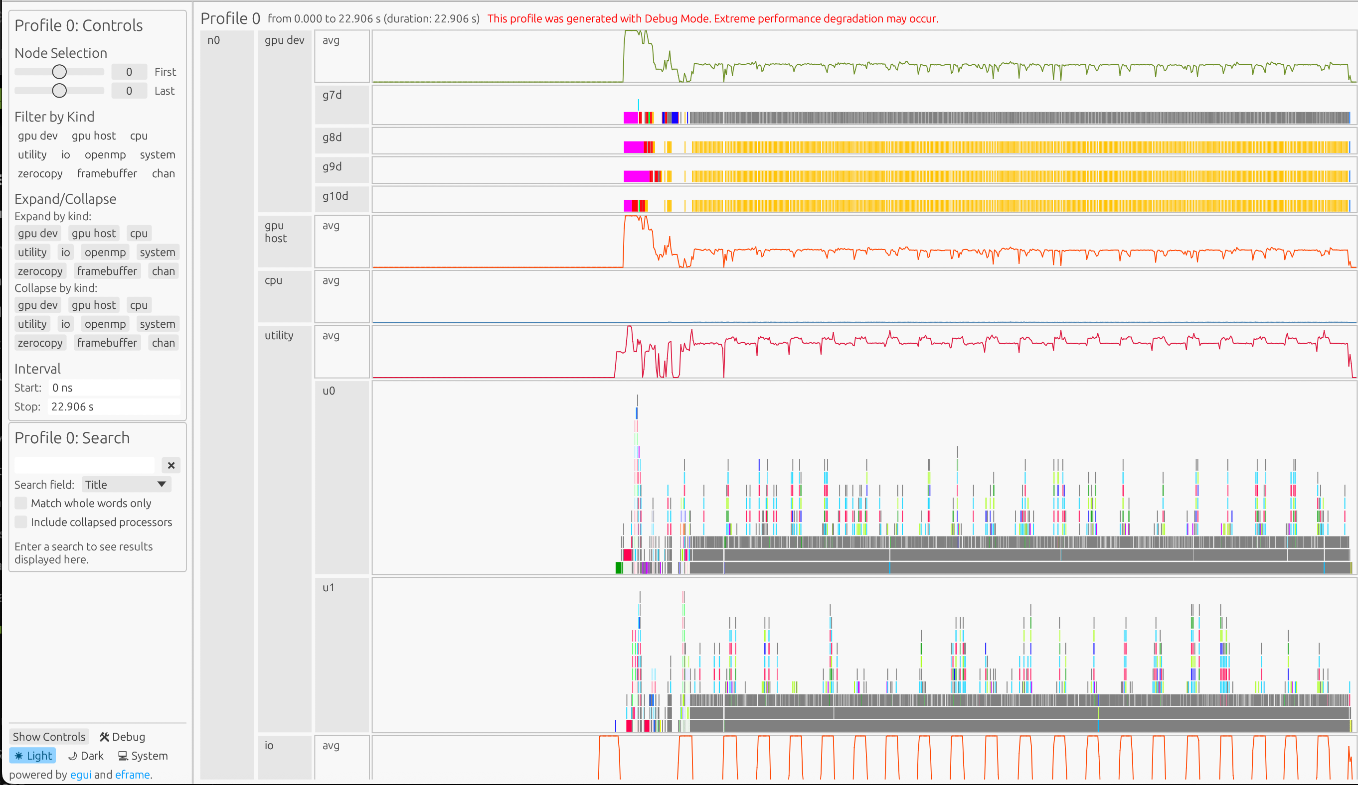
The viewer will open a window with a timeline of your program’s execution:

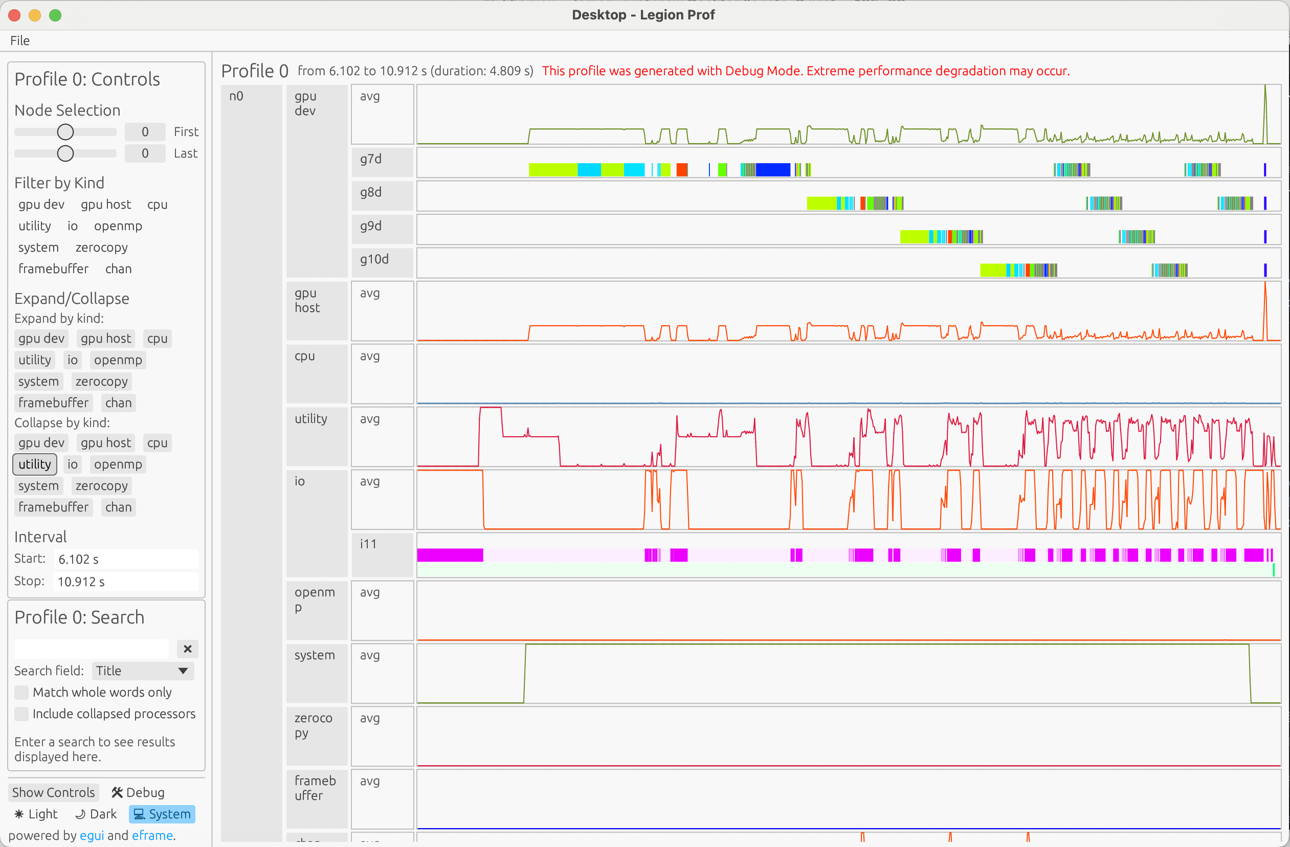
Understanding the Profile

Each node appears as a separate section in the UI, with a timeline showing the execution of tasks on that node. Within each timeline, you’ll see different substreams for processor execution and memory utilization over time. Each box represents either a task (on processor streams) or an instance/memory allocation (on memory streams).

Processor and Memory Stream Types

Stream Type	Parameter	Description
CPU	--cpus	Main CPU cores for user tasks, computations, and data movement
GPU Device	--gpus	GPU execution units for CUDA kernels, GPU memory operations
GPU Host	(automatic)	Host operations for GPU tasks
Utility	(automatic)	Dedicated CPU cores for runtime meta-work such as task mapping, dependency analysis, and coordination
OpenMP	--omps, --ompthreads	OpenMP thread pools for parallel CPU execution, loop parallelism
IO	(automatic)	File I/O operations, Python execution time, other TopLevelTask-level operations
System	(automatic)	Low-level system interactions such as memory allocation, process/thread management, and kernel operations
Zero Copy	(automatic)	Zero-copy memory allocations/deallocations
Framebuffer	(automatic)	Framebuffer memory allocations/deallocations
Channel	(automatic)	Communication pathways grouped by source and destination memory of copies, showing copy information such as timing and instances.

Interpreting Stream Activity

You can interact with the timeline by clicking on different elements:

• Click on task boxes to see detailed execution information

• Click on substreams to expand and see all tasks for that processor type

• Hover over task boxes to see summary information like task names, duration, and status

Task box colors represent the current state of each processor:

• Darkest shade: Task is actively executing on the processor

• Intermediate shade: The event that the task blocked on has triggered, so the task is ready to resume execution, but it hasn’t started yet (most likely because another task is currently executing on the processor). If this is the case, the “Previous Executing” field will tell you which task was preventing the ready task from resuming.

• Lightest shade: Task is blocked waiting on an event and has been preempted which means that it is not running and the event that it blocked on has not yet triggered

• Empty spaces: Processor is idle with no tasks scheduled

• Gray sections: Groups of very small tasks that are too small to display individually at the current zoom level

The relative activity and idle time across different streams can help identify performance bottlenecks:

• High CPU utilization with low GPU usage may indicate insufficient GPU work

• Busy utility processors suggest the runtime is working hard on scheduling

• Frequent and long operations in Channel might indicate data movement bottlenecks

• Long IO operations suggest you are waiting on Python code to be executed first

• Gaps between tasks on the same processor may reveal synchronization issues

• It can also reveal that your program has a dependency on long copies, a utilility thread that is too busy, or other issues.

If you want to understand why a specific box on the profile timeline didn’t start executing earlier, you can look at the “Critical Path” field on the pop-up box for more information.

Example: Conjugate Gradient Algorithm

To demonstrate these profiling concepts in practice, let’s examine a real-world example using the Conjugate Gradient (CG) algorithm. This algorithm solves linear systems of the form Ax = b where A is a symmetric positive definite matrix. The implementation of the CG example is available here.

The profile below shows the CG example running on a system with 4 GPUs:

Key Observations

To understand a program’s behavior and investigate bottlenecks, we often inspect GPU tasks, utility processors, and communication channels.

GPU Tasks

In the CG code, the workflow begins with matrix generation and variable initialization, followed by warmup iterations, and then the main iterative algorithm (which includes matrix-vector multiplications and dot products) until convergence. In the GPU Device stream, we can see that:

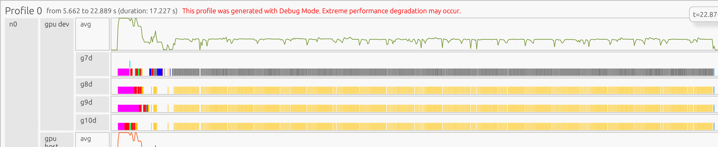
• Initial operations appear slower due to one-time CUDA setup costs (context initialization, memory allocation, and kernel compilation). This startup overhead is expected and unrelated to cuPyNumeric performance.

• Post-warmup iterations show faster and more consistent execution as the runtime reaches steady state, with uniform kernel durations indicating efficient reuse of compiled kernels and allocated memory.

• The program concludes with tasks that unload the CUDA libraries on each GPU (the blue boxes at the end of the timeline)

If you zoom in, you can see iteration-level patterns:

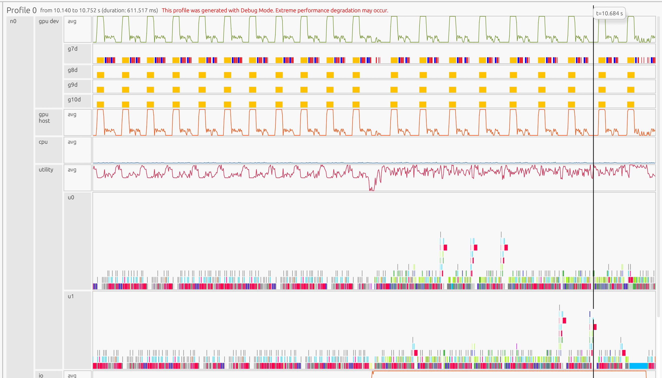
In the GPU Device stream, the yellow boxes are cuPyNumeric matrix-vector multiplication task kernels, the blue boxes are cuPyNumeric dot task kernels, and the red boxes are cuPyNumeric binary operation task kernels.

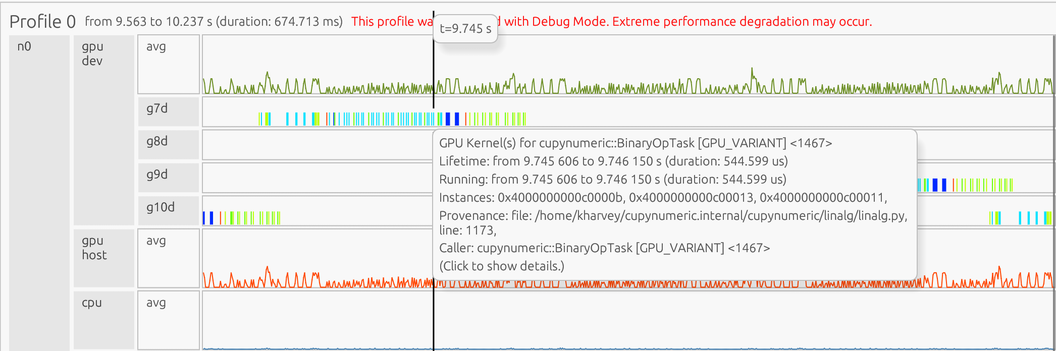
Clicking on a box in the profile opens a pop-up showing detailed information about that task:

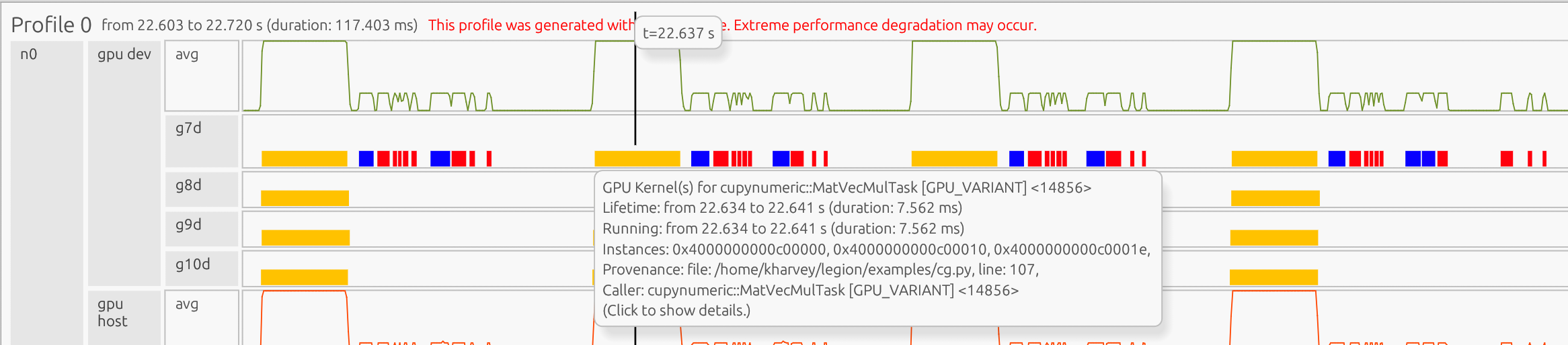
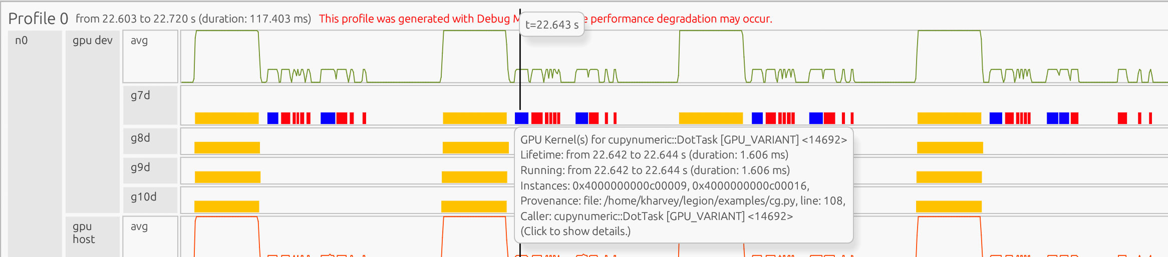
The pop-up shows that the matrix-vector multiplication task corresponds to line 107 and the dot task corresponds to line 108 in the code:

107 Ap = A.dot(p)
108 alpha = rsold / (p.dot(Ap))

Utility Processor

The utility processor shows Legate runtime behavior, including task mapping, dependency analysis, and scheduling. In this example:

• Busy utility processors indicate active optimization of task placement and data movement

• Gaps between GPU tasks often correspond to runtime mapping and scheduling activity. They may also indicate the GPU is waiting for other operations to complete (i.e. memory copies)

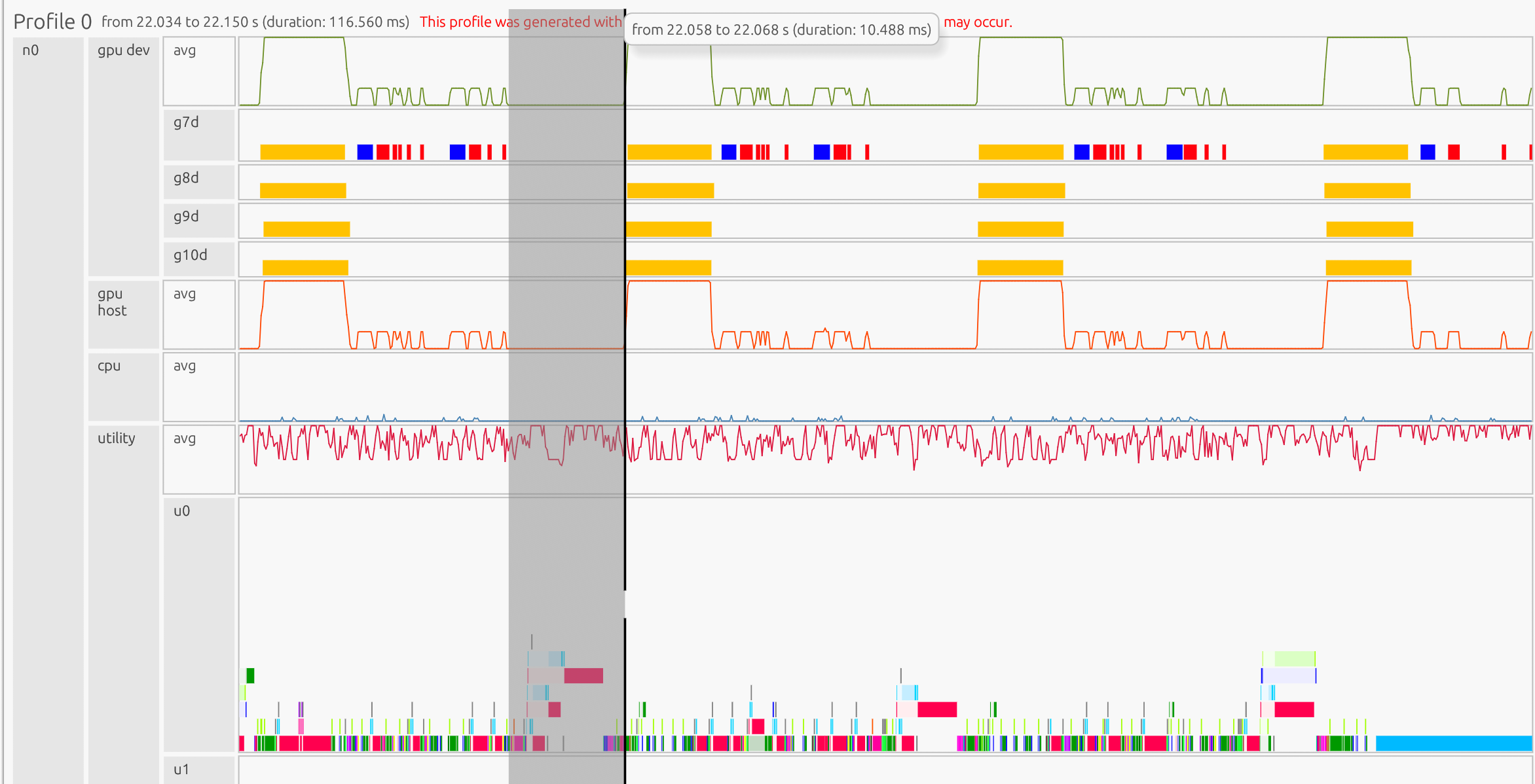
The utility processor shows that the gap between the matrix-vector multiplication (line 107) and the dot task (line 108) occurs because the dot task depends on the completion and mapping of the result of the matrix-vector multiplication.

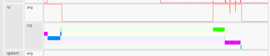
Communication Channels

The communication channels show data movement patterns between devices:

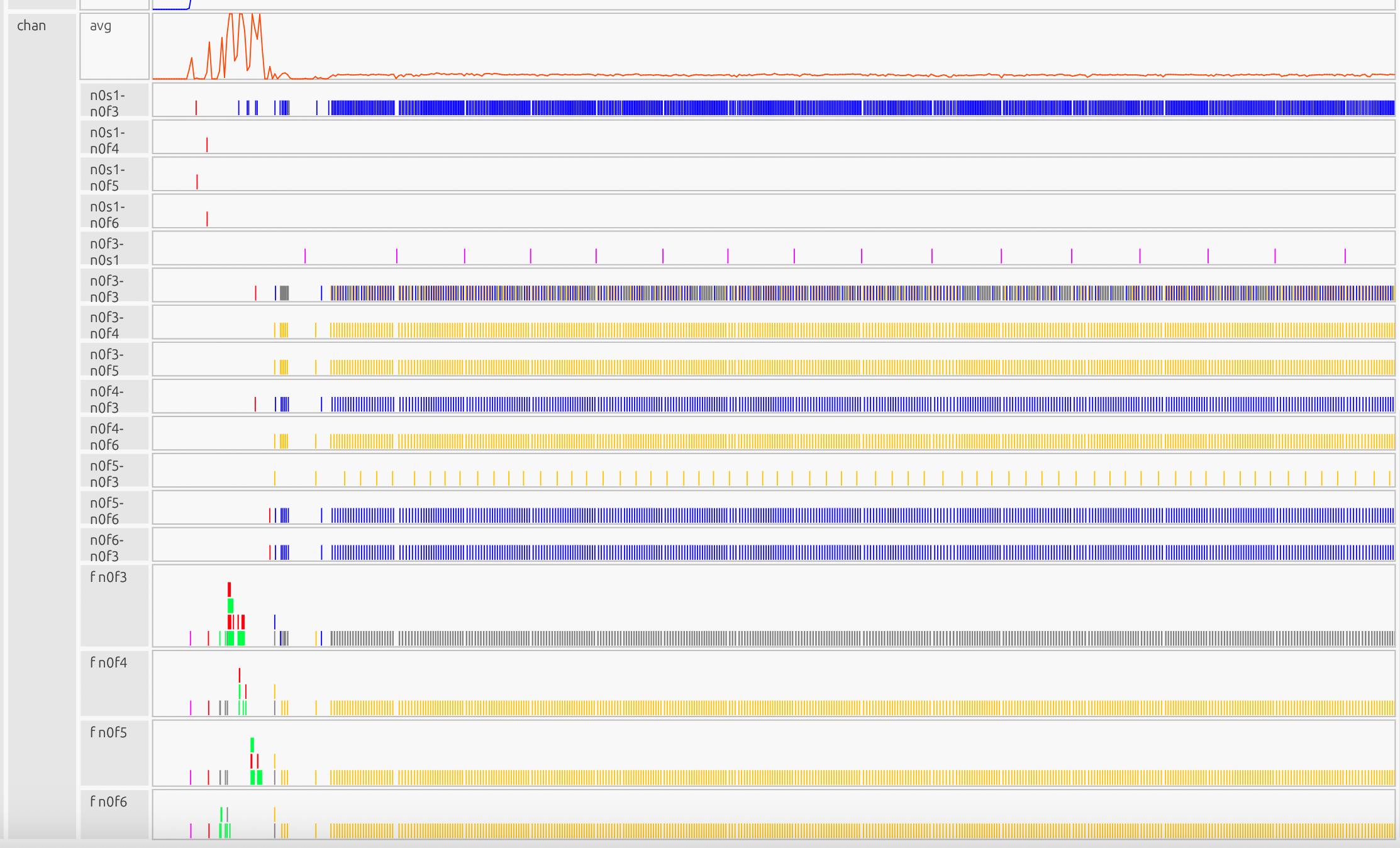
At the start of the program, device-to-device copies are sparse due to initialization and warmup iterations, but they become more uniform in subsequent iterations. The length and frequency of these transfers indicate whether data is moved in large chunks or in smaller, more granular batches.

Applying this to your own program

When profiling your own program, you can look at the same streams to better understand its behavior and locate potential bottlenecks:

• GPU stream: Identify unusually long tasks and inspect the corresponding code to determine if an operation is taking longer than expected. Note any gaps between GPU tasks and check which other streams are active during those gaps

• Utility processor: Monitor utility processor activity, as lower usage typically indicates better performance. When utility processors are constantly busy, this suggests the runtime is spending excessive time on task scheduling and coordination. To address this, consider coarsening your tasks by processing larger data chunks per task or fusing multiple operations together. For applications with repeated loops, enabling tracing can significantly reduce utility processor overhead. Additionally, if utility processors remain overly busy, you should examine mapper call lifetimes to ensure your mapper isn’t spending too much time making decisions

• Channel stream: Review data transfers between devices to understand their timing, purpose, and potential impact on performance

When comparing different versions of the same application, you can compare how these metrics change between runs.

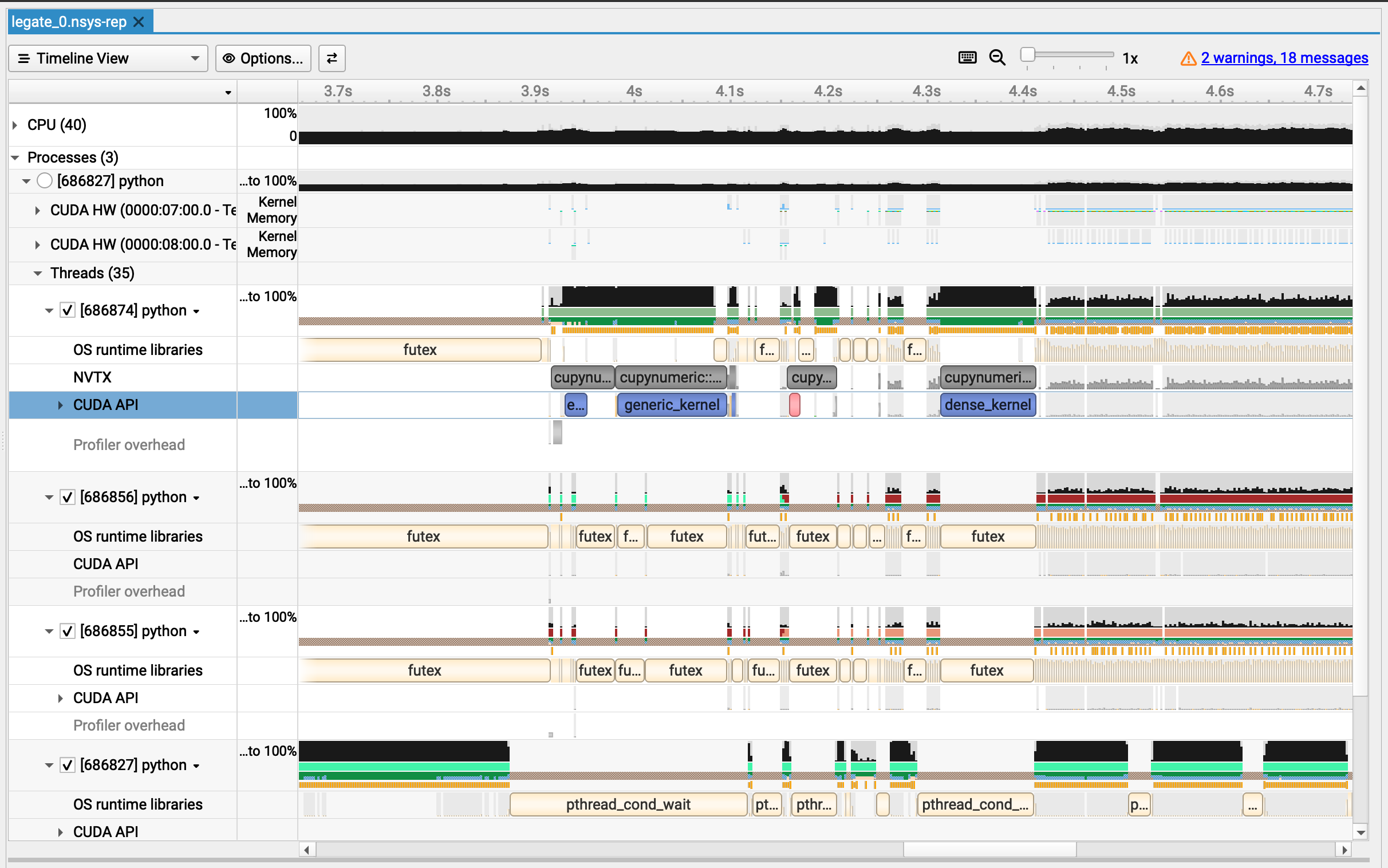
Integrating with NVIDIA Nsight Systems

Below are the steps necessary to build and run the Legion Prof tool, profile a Legion program, and export profiling data through NVTXW, which can then be viewed in NVIDIA Nsight Systems 2024.5.1 or later.

Setup Nsys/Legion Prof

First, install NVIDIA Nsight Systems 2024.5.1 or later. It is available from: https://developer.nvidia.com/nsight-systems/get-started#Linuxx86

Building with packages

If you want to install with pip, you can do so with:

pip install legate-profiler

Otherwise, you can install with conda:

conda install -c conda-forge -c legate legate-profiler

Run Nsys/Legion Prof

With all prerequisites built, you can now run Legion programs to profile them.

A sample command using Legion’s CG example would be:

legate --gpus 2 --nsys --profile examples/cg.py  -n 235

This will create a legate_0.nsys-rep file which can be viewed in the Nsight Systems UI. In this file, you can see your cuPyNumeric operations in the NVTXW row: